
[et_pb_section fb_built=”1″ _builder_version=”3.0.47″][et_pb_row _builder_version=”3.0.48″ background_size=”initial” background_position=”top_left” background_repeat=”repeat”][et_pb_column type=”4_4″ _builder_version=”3.0.47″ parallax=”off” parallax_method=”on”][et_pb_text _builder_version=”3.0.74″ background_size=”initial” background_position=”top_left” background_repeat=”repeat”]
Excel macros are like mini-programs that perform repetitive tasks, saving you a lot of time and typing. For example, it takes Excel less than one-tenth of a second to calculate an entire, massive spreadsheet. It’s the manual operations that slow you down. That’s why you need macros to combine all of these chores into a single one-second transaction.
Excel macros: Tips for getting started
We’re going to show you how to write your first macro. Once you see how easy it is to automate tasks using macros, you’ll never go back.
First, some tips on how to prepare your data for macros:
- Always begin your macro at the Home position (use the key combination Ctrl+ Home to get there quickly).
- Use the directional keys to navigate: Up, Down, Right, Left, End, Home, etc., and shortcut keys to expedite movement.
- Keep your macros small and focused on specific tasks. This is best for testing and editing (if needed). You can always combine these mini-macros into one BIG macro later once they’re perfected.
- Macros require “relative” cell addresses, which means you “point” to the cells rather than hard-code the actual (or “absolute”) cell address (such as A1, B19, C20, etc.) in the macro. Spreadsheets are dynamic, which means they constantly change, which means the cell addresses change.
- Fixed values and static information such as names, addresses, ID numbers, etc. are generally entered in advance and not really part of your macro. Because this data rarely changes (and if it does, it’s just to add or remove a new record), it’s almost impossible to include this function in a macro.
- Manage your data first: Add, edit, or delete records, then enter the updated values. Then you can execute your macro.
Why starting with mini-macros is easier
For this example, we have a store owner who has expanded her territory from a single store to a dozen in 12 different major cities. Now the CEO, she’s been managing her own books for years, which wasn’t an easy task for a single store, and now she has 12. She has to collect data from each store and merge it to monitor the health of her entire company.
We created a few mini-macros to perform the following tasks:
- Collect and combine the data from her 12 stores into one workbook in a Master three-dimensional spreadsheet.
- Organize and sort the data.
- Enter the formulas that calculate the combined data.
Once the mini-macros are recorded, tested, and perfected, we can merge them into one big macro or leave them as mini-macros. Either way, keep the mini-macros, because it’s much easier and more efficient to edit the smaller macros and re-combine them, than try to step through a long, detailed macro to find errors.
We’ve provided a sample workbook for the above scenario so you can follow along with our how-to. Feel free to create your own spreadsheet too, of course.
Prep work: The Master spreadsheet
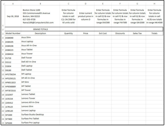
If you’re building your spreadsheets from the ground up, start with the Master spreadsheet. Enter the date formula in A1 and the store location in B1. See screen shot below.
Enter this date formula in cell A1: =Today(). Now this cell always displays today’s date. Be sure; however, that your store location (branch name and number) are entered in B1.
2. Leave row 2 blank. Once the static data and initial dynamic data are entered, we’ll use row 2 for the totals. This might seem like a strange custom, but for macro spreadsheets, it’s the best way because this row is stationary and always visible.
3. Next, enter the field names (and/or any other field-specific information) in row 3 (e.g., from A3 through J3, or however many fields your spreadsheet requires).
Tip: You can text-wrap the information in the individual cells if the data is lengthy. For example, you can put the store contact information all in one cell and wrap the lines. Press Alt+ Enter to insert extra lines in the cells.
4. Next, enter the static data in column A. That is the record information in your spreadsheet that rarely changes. If your business uses product numbers or ID codes, which are unique because there is only one code per product, enter those in column A beginning on row 4 (don’t skip to row 5). Other static data fields might include the Product Description, the Product Price, sales tax percentage, etc.
Do not skip rows or leave any rows blank for column A. Every row must contain the unique field’s data—if not a product code, then some other unique identifier. We do this for two reasons:
- Column A is the main navigational column. The macro moves and navigates through the spreadsheet based on the Home (A1) position and column A. The macro will fail if you ignore this rule, because blank rows disrupt the actions of the directional keys.
- If you decide to create multiple/relational tables later for Pivot Reports, you must have a unique, key field to connect the related tables. Check out our Excel pivot tables tutorial for more information.
Build the Master spreadsheet first.
5. Normally, the Product Description resides in column B, the Quantity Sold in column C, Product Price in column D, Extended Cost in E, Discounts in F, Sales Tax in G, and Totals in H. The column totals are across the top on row 2, remember? Format the column widths based on the length of the field names, and adjust the row height to 20 on all rows. Change the Top/Bottom alignment to Center, select the justification you prefer (left, right, center), and then format the spreadsheet “styles” to your preference.
6. Once the master database is set up, do not move anything. If you need to add fields, use the Insert Column command. For example, if you wanted to add a second sales tax, position your cursor anywhere on column H (Totals) and click the tab: Home > Insert > Insert Sheet Columns. The new column drops in to become the new H column, and the Totals column moves over to I. This process does not affect the macro.
7. The same process applies to rows. Normally I would caution you to insert rows “inside” the active database area. For example, if the formula says =SUM(B3:B20) and you insert or use a row outside of the formula’s range like B21, the new record’s data is not included in the formula and therefore, does not calculate.
8. Now we’ll set up that formula range. Enter the following formulas on row 2 (this is a one-time task):
C2: =SUM(C4:C500)
E2: =SUM(E4:E500)
F2: =SUM(F4:F500)
G2: =SUM(G4:G500)
H2: =SUM(H4:H500)
Next, enter the following formulas in these columns (also a one-time event):
E4: =SUM(C4*D4), then copy from E4 down to E5:E500
F4: =SUM(E4*10%), the current discount percentage in your store, then copy from F4 down to F5:E500
G4: =SUM(E4-F4)*6.25, where 6.25 is the sales tax in your area, then copy from G4 down to G5:G500
H4: =SUM(E4-F4+G4), then copy from H4 down to H5:E500
Now that you have all the spreadsheet formulas in place, all you have to do is enter the quantity (column C) for each computer sold (daily, weekly, or monthly). If the prices change, enter the new prices in column D. The rest of this database is all formulas or static information.
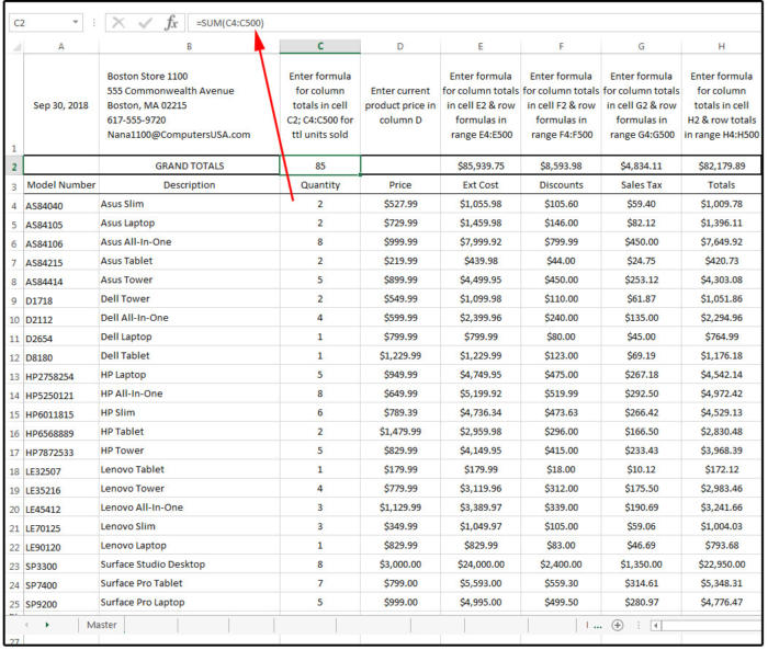
Enter the formulas to calculate the columns and rows.
9. As seen above, with “macro” spreadsheets, you set the formula range to be many rows beyond the last record, so you can just add new records at the end and not worry about adjusting the range. Because the macro sorts the database, the new records are relocated to the proper position. The spreadsheet data in our example ends on row 210. The formula range extends out to row 500, so it’s safe to add the next new record on row 211.
10. Once the spreadsheet is defined and set up with the structure, static data in place, and correct formulas, make 12 copies in worksheets 2 through 13. Edit the tabs on the bottom to identify the individual stores. Change the name of the sheet1 tab to Master, because this is your master database file.
11. Change the location data on row 1 to identify the store information (that matches the store on the tab) on all 12 spreadsheets. Next, email an electronic copy of each branches’ spreadsheet to each of the store managers; for example, send the Boston sheet to Boston, the the Dallas sheet to Dallas, etc.
Their copies include the spreadsheet formulas that work on their individual spreadsheets (but not the formulas of the combined spreadsheets in the workbook).
12. The macro provides the formulas for the Master. The Master is the spreadsheet for the combined totals of all stores. If you are the one who collates all the data and executes the Master macros AND you also manage an individual store, you must use one of the 12 sheets you copied for your store. The Master is for the grand totals only.
13. Once the branches email their individual spreadsheets, it’s safer to just copy the individual sheets from the 12 stores’ workbooks manually.
Copy the Master spreadsheet 12 times, then name the tabs.
Macro1: Collect and combine data
1. Access your database folder and open your spreadsheet titled MasterDB.xlsx
2. Open one of the new store spreadsheets, such as the one titled BostonDB.xlsx
3. Move your cursor back to the MasterDB so it’s the active sheet.
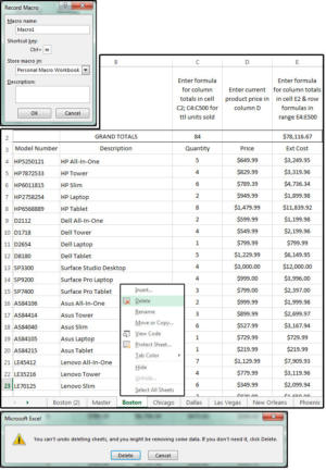
4. Select the Developer tab and click Record Macro or press ALT+ L+ R. The Macro Name field says Macro1, and that’s a good name.
5. Enter a shortcut key (if you like) in the Shortcut_key field box (enter the letter M) (you can create a button on the Ribbon menu later).
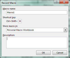
Record macro dialog box, macro shortcut_key
6. In the Store Macro In field box, click the down arrow and select Personal Macro Workbook from the list, then click OK.
Now you are recording the macro.
Follow the instructions below, exactly, and use your mouse to navigate around the spreadsheet. Please note that phrases inside square brackets are tips, notes, and explanations of the instructions. Do not include these phrases or anything they say in your macro.
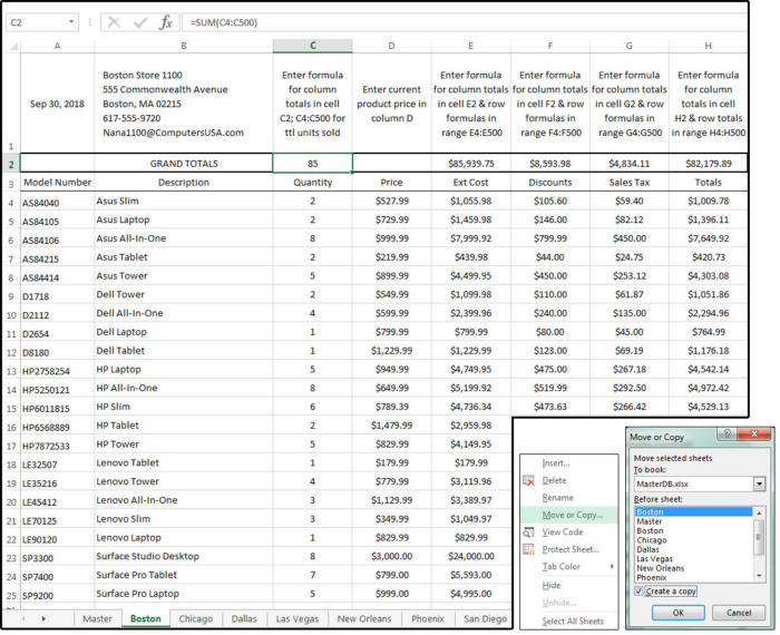
1. Move back to the BostonDB spreadsheet, then right-click the Boston tab. In the popup menu, select Move or Copy …
2. In the Move or Copy dialog, check the box that says Copy.
3. In the Move Selected Sheets dialog, click the down arrow beside the To Books field box.
4. Select “MasterDB.xlsx” from the list.
5. In the second dialog: Before the Sheet, select the first spreadsheet on the list called “Master,” then click OK.
8. Excel copies the sheet and relocates your cursor to the MasterDB. Notice the new tab that says “Boston2.” Verify that the info in cell A1 shows the store number followed by a recent date (9/29/18 in this example). If yes, you’re good to go.
9. Right-click the tab of the original Boston spreadsheet and select Deletefrom the popup menu.
10. Excel warns in a dialog box: You Can’t Undo . . . Delete or Cancel? If you’re certain you want to remove it click Delete.Why? Because you want to replace it with the NEW Boston sheet that the Boston manager sent to you.
11. Move the Boston2 tab between the Master and Chicago tabs. If you keep the ‘2’ from Boston2, it will be easier to quickly recognize which sheets have been updated each month.
13. Click Ctrl+ Home to relocate cursor to cell A1 and re-enter this date formula: =TODAY(), (if this formula is missing), then press the Enter key
Record the macro, combine the data, delete duplicate sheets
Execute the Macro
1. Select the Developer tab again and click Stop Recording or press ALT+ T+ M+ R.
2. Save the Master file, then save the BostonDB file.
3. Go back to the MasterDB spreadsheet and run the macro: Press Ctrl+ M.
NOTE: Remember that the ‘+’ sign means a “simultaneous” combination keystroke; that is, Ctrl+ Shift- Jmeans: Press and hold down the Ctrl and Shift keys with your left hand, then press the J key with your right hand, then release all three keys simultaneously. The dash (or hyphen) means a “consecutive” combination keystroke, such as End- Down, which means press the End key and release, then press the Down arrow and release. These are NOT interchangeable, so watch the signs.
4. If the macro works as expected, repeat this process again for each of the remaining 11 spreadsheets, then run the macros, save the files, and exit all spreadsheets except the Master.
NOTE: The only available shortcut keys are Ctrl+ M (which you have already used), Ctrl+ Shift- M, Ctrl+ J, and Ctrl+ Shift- J. Because shortcut keys are in short supply and the character combinations don’t make any logical sense anyway, the best solution for your mini macros are macro buttons on the Ribbon menu with names that make sense, such as Boston for the Boston macro and Dallas for the Dallas macro. Check out this other Excel macros how-to, where there’s a section with detailed instructions on how to create, name, and use macros.
Macro2: Organize and sort data
This one is easy, but with so many spreadsheets, it can be a daunting task if you do it manually. Excel actually provides a way to modify all your spreadsheets at once, but this task is unreliable when sorting.
Follow the Record Macro instructions (4, 5, 6 under Macro1 above) to create this next macro. Name the macro Macro2 and use Ctrl+ Shift- M for the shortcut (you can create a button on the Ribbon menu later). This macro affects all the spreadsheets in the MasterDB, so ensure this file is open and active.
1. Press Ctrl+ Home [to move cursor to A1].
2. Press the Down arrow key three times.
3. Press Shift- End- Down- End- Right [Hold down the Shift key, press the End key and release, press the Down Arrow and release, press the End key and release, press the Right arrow and release all].
4. Select Data > Sort. In the Sort dialog, choose Model Number from the drop-down list in the Sort By field box, then choose Values from the Sort Onfield box, and then choose A-Z from the Sort Order field box, and click OK.
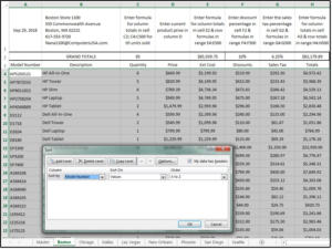
Macro sorts the spreadsheet by Model Number
5. Press Ctrl+ Home.
6. Click the next tab at the bottom to access the next spreadsheet (i.e., Chicago after Boston), and repeat all steps above: 1-6, and then continue with the following instructions below. Remember, the macro is recording through all these steps.
7. Click the Master spreadsheet tab, press Ctrl+ Home.
8. Select the Developer tab (from Ribbon menu) and click Stop Recording or press ALT+ T+ M+ R.
9. Save the Master file, MasterDB.
10. With cursor still in MasterDB spreadsheet, run the macro: Press Ctrl+ Shift- M.
Macro3: Enter formulas
The formulas for the individual stores’ spreadsheets are already in place. You entered those back in step #9 of the Prep Work section above. These formulas are for the Master spreadsheet, which calculates all the others and combines the grand totals into one “master” sheet. We use a macro for this process rather than doing it manually 12 times.
Follow the Record Macro instructions (4, 5, 6 under Macro1 above) to create this next macro. Name the macro Macro3 and use Ctrl+ J for the shortcut (you can create a button on the Ribbon menu later). This macro affects all the spreadsheets in the MasterDB, so ensure this file is open and active.
1. Press Ctrl+ Home [to move cursor to A1].
2. Press Down- Right- Right
3. =SUM(Boston:Denver!C2) Enter [Enter this formula in cell C2, where the tabs named Boston and Denver represent the first and last spreadsheet tab names in your workbook. This is excluding the Master, of course, because you are calculating all the values in cell C2 from the first tab Boston through the last tab Denver and entering the totals in cell C2 of the Master. Then Enter key is pressed).
4. Up arrow, Ctrl+ C [Moves cursor back up to cell C2 and copies this formula]
5. Right- Right- Shift- Right- Right- Right Enter [moves cursor to the right twice and stops on cell E2, press the Shift key and hold down while moving to the right three times, which highlights cells E2 thru H2, then press the Enter key].
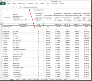
Enter+ calculate formulas in Master for multiple sheets
6. [While these cells are still highlighted, press] Shift- Ctrl+ 4
7. ALT+ T+ M+ R [Press these keys simultaneously or select the Developer tab and click Stop Recording].
Save, copy, and distribute
1. Ctrl+ Home
2. Save the Master file, MasterDB.
3. Send copies of the MasterDB to all store managers.
This article was originally published on PCWorld byJD Sartain.
[/et_pb_text][/et_pb_column][/et_pb_row][/et_pb_section]